Tutorial

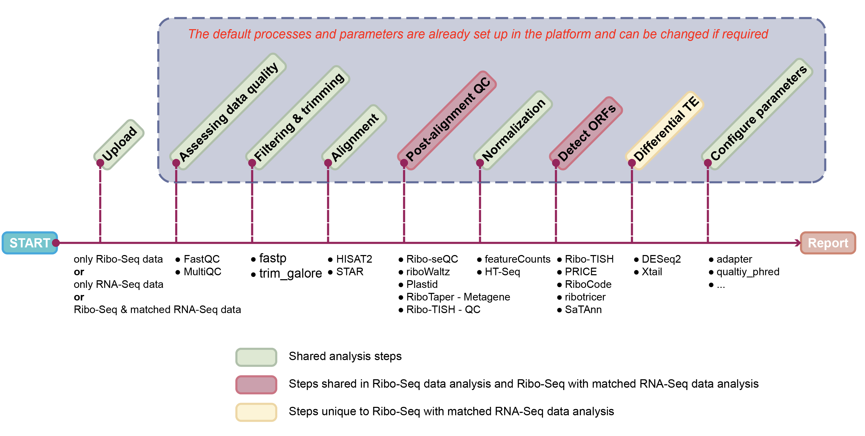
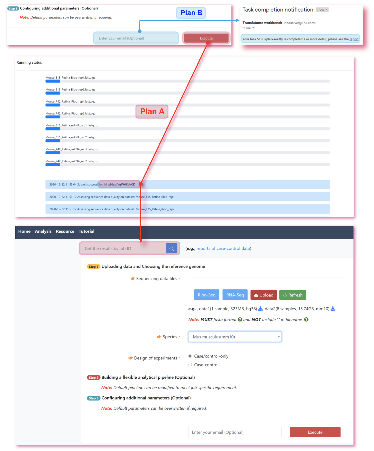
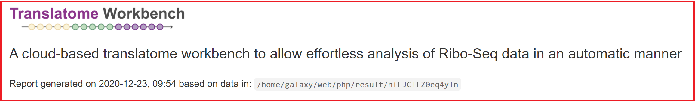
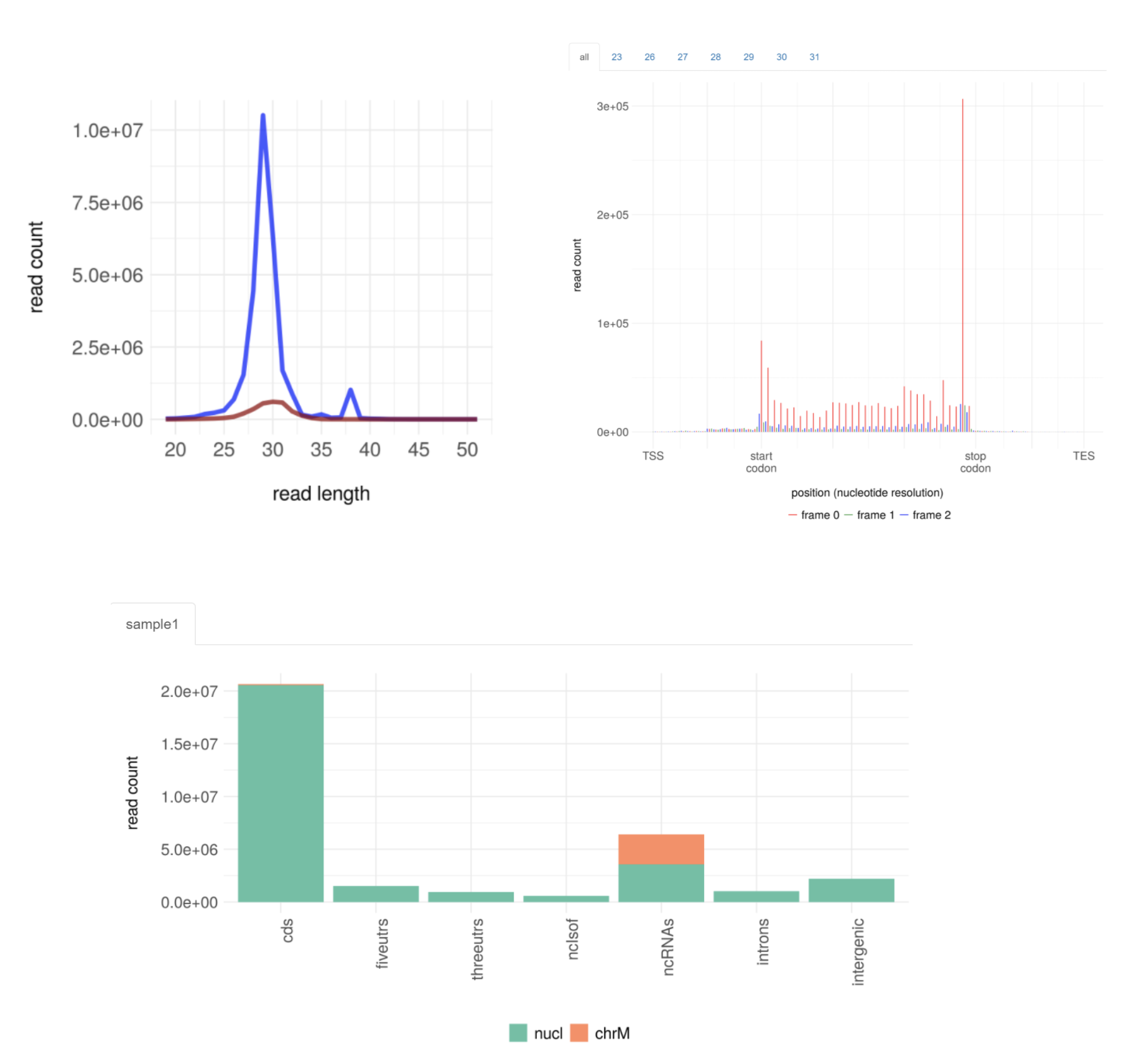
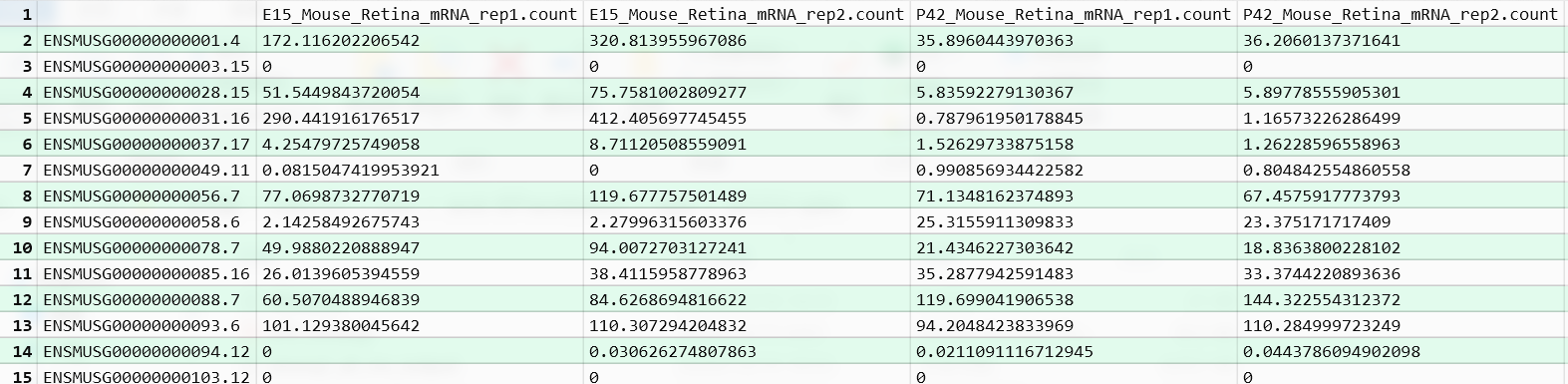
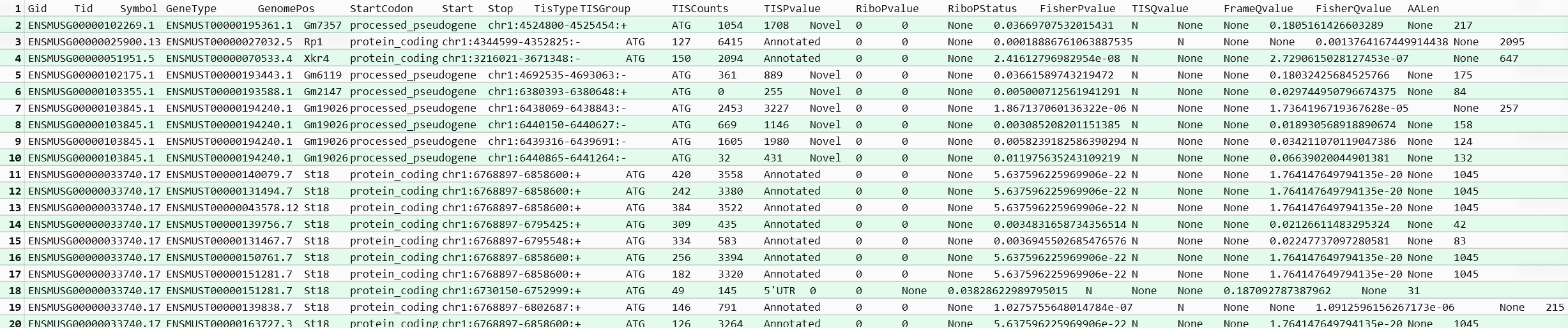
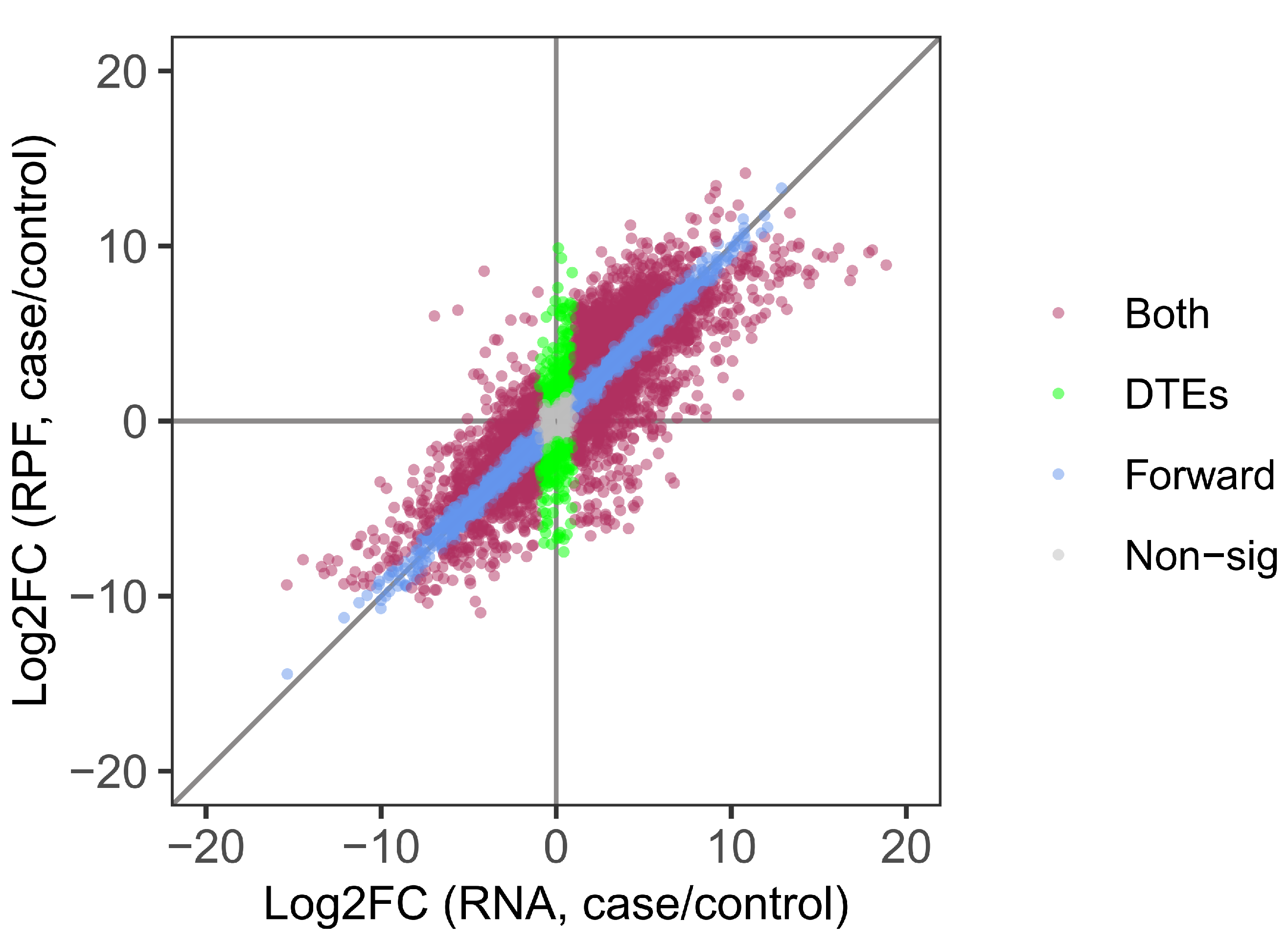
The translatome workbench is a convenient, freely available, web‑based platform to allow effortless analysis of ribosome profiling data in an automatic manner for experienced bioinformaticians, as well for wet‑lab biologists with minimum bioinformatics knowledge. It embeds more than 20 popular analytics tools that provides a full pipeline to cover all key steps for ribo‑seq data analyses, from raw read mapping, filtering and normalization, to the computation of translation‑associated contents such as offset estimation, triplet periodicity, actively translated ORFs detection, and finally to the visualization of analysis results, along with a document report. Additionally, considering that Ribo‑seq and RNA‑seq are often sequenced in parallel, it can also be used to carry out the processing of RNA‑seq data and the integrated analysis of Ribo‑seq and RNA‑seq data, such as differential translational efficiency analysis. Overall, this web server will bring an unprecedented level of convenience for the researcher to decipher information embedded within Ribo‑seq data. upload


First, we need to upload and set up information about the analysis data. As mentioned above, translatome workbench can analyse both Ribo-Seq and matched RNA-Seq data. Therefore, we will use the mouse retinal data (Ribo-Seq and mached RNA-Seq data, divided into two groups, E15 and P42, each with two replicates) as an example to show step by step how to use translatome workbench.

(1) Click on Ribo-Seq to select the data to be analysed, here it refers to Mouse_E15_Retina_Ribo_rep1, Mouse_E15_Retina_Ribo_rep2, Mouse_P42_Retina_Ribo_rep1, Mouse_P42_Retina_Ribo_rep2

(2) Click on RNA-Seq to select the data to be analysed, here it refers to Mouse_E15_Retina_mRNA_rep1, Mouse_E15_Retina_mRNA_rep2, Mouse_P42_Retina_mRNA_rep1, Mouse_P42_Retina_mRNA_rep2

(3) Click on Upload to upload the data after confirming that it is correct, the upload progress will be displayed with a blue progress bar; if incorrect, click on Refresh to reselect the data

(4) Click on Species drop-down field to select the appropriate genome (in this case it is the choice of mm10). A certain genomic index have been built into our platform, such as hg19, hg38, mm10, etc.

(5) Experimental design: Choose Case-control as this example contains two groups of data and a form will then pop up that requires information about the data to be uploaded. If there is only one condition for uploading data, then only the Case/control-only needs to be clicked.

  • In Group 1, enter the name of the first group of sequencing data in the second column of the table, represented here by E15, the data framed by the red background in the figure below, and set custom names for each of them in the first column; click on the 'plus' or 'minus' buttons on the right to increase or decrease the data
  • In Group 2, set up the second group of data in the same way as above, that is, the data with the blue background shown below
  • The name of the data entered in the second column of the table must have the same prefix as the name of the uploaded data

step1


Note: Step2 and Step3 have been configured with default processes and parameters, which can be changed by the user as required.


After uploading and setting up the condition information for the data, the next step is to process the data for analysis. This step automatically sets up an adapted analysis process depending on the type of data uploaded and the type of experimental design. Therefore, in general, no additional settings are required for this step. Of course, the default options can also be replaced by mouse clicks.

step2

  1. filtering and trimming
    • adapter: the adapter sequence used for sequencing
    • quality_phred: minimum sequencing quality of the retained reads
    • length_required: the minimum length of the reads after trimming adapter and low quality bases
  2. alignment
    • MismatchNmax: the maximum number of base mismatches per read
    • MultimapNmax: maximum frequency of alignment to multiple positions per read
  3. footprint length
    • min_length: the minimum retention length of reads derived from Ribo-Seq data
    • max_length: the maximum retention length of reads from Ribo-Seq data
  4. differential cutoff
    • adjusted_pvalue: Significance threshold setting for corrected p-values in differential translational efficiency analysis
    • log2FoldChange: threshold value for log2 transformed fold change in differential translational efficiency analysis
3 parameters
Finally, there are two options for executing and accessing the results. Plan A if no suitable email address is available for receiving results; and Plan B to receive the results report via email.
Plan A
  1. NOTE! After clicking on Execute button, the unique identifier, job id, of the process will appear, please keep it safe for downloading the result data!
  2. Data processing progress will be displayed in real time at the bottom of the page.
  3. Once the analysis has been completed, the job can be searched for and the report retrieved from the search box at the top of the analysis page using the job id.
Plan B
  1. Enter the email address to the box next to the Excute button. Then click on the Execute button and the progress of execution will be displayed in real time at the bottom of the analysis page
  2. Once the process has been executed the report will be automatically sent to the email address you have entered and you can then download the report by clicking on the link in the email address. If the analysis page shows that the execution is complete but you do not receive the email, then please check in the spam folder.

4 execute

The execution report generated in the previous step nests all the results of the analysis process in an html format for easy viewing by the user. In addition, the results of each step are extracted separately from it. Below we have presented and contextualised the results of each section.

report
Being different from RNA-seq data, Ribo-Seq data seems more sophisticated, which are not only reflected at experimentation but also data analysis. A crucial step in the Ribo-Seq data analysis is quality control during pre-processing, which reflects whether sequencing is high-quality and is also the foundation for subsequent analysis accurately. 2.1 FastQC
The length of reads from Ribo-Seq generally falls in the range of 25nt to 35nt as they are enclosed by the ribosomes. Therefore, only trimmed reads in this interval will be retained for subsequent analysis on account of excluding reads stemmed from contaminations. Additionally, rRNA and tRNA are also required to be removed for improving mapping ratio and accelerating subsequent analysis in the pre-processing. Two types of software, fastp and trim_galore, are provided here for use. 2.2 QC
Tools used to mapping RNA-Seq data are also adapted in alignment of Ribo-Seq data, such as HISAT2, STAR, TopHat2. Through mapping reads against to the reference sequences, we can know which genes are expressed and how the expression of them. Following gene functional analysis, we could learn more about what effects are caused by the experimental treatment. 2.2 alignment
A few unique features of Ribo-Seq data, for example, distribution of read length and triplet nucleotide periodicity, can be detected from BAM files, which are generated by alignment. First, Sequencing reads of Ribo-Seq data are from fragments of ribosome-enclosed, so the distribution of read lengths will mainly concentrate on a specific length. Second, the most significant feature of Ribo-Seq data is triplet nucleotide periodicity and this feature is also the criterion to judge the quality of Ribo-Seq data. If we can't observe this feature, we should reflect on reasons leading to these results. For example, whether there is an error during the library preparation. If the triplet nucleotide periodicity can not be observed after we rule out all of the points that we may make an error, we should consider to drop out this data. Third, sequencing reads from Ribo-Seq data are usually located in the translated genomic regions. However, reads resided in the UTR or intronic regions are also worthy of attention due to their underlying regulatory functions. For example, it is likely that the expression of 5'UTR on the gene displayed in the figure below inhibited the expression of CDS, however, this phenomenon is not observed within the RNA-seq data. Hence, the distribution of reads on the genomic features provides new insight into the regulatory mechanism of gene expression. 2.3 post-align-qc
After pre-processing is completed, BAM or SAM format files will be obtained for follow-up analysis, from which we can get exactly counts of reads for each gene utilizing tools like featureCounts. Nonetheless, it is necessary taking into account of library size if we need to compare differential expression of interesting genes. In other words, normalization of gene counts is requisite prior to differential expression analysis. Hence, we provide two options, RPKM and TPM, for normalizing the read counts. 2.4 normalization
Ribosome profiling provides us a unprecedent opportunity to detect actively translated ORFs in a more accurate manner. Thus, previous studies have identified a plethora of ORFs with ribosome profiling such as small open reading frames (smORFs), upstream open reading frame (uORFs). Detection of ORFs is a characteristic and significant analytical aspect in translatomics analysis. Given that reads from Ribo-seq are mainly derived from region of ribosome protected, we can infer underlying actively translated regions from the profile of mapping results by feat of relevant tools like Ribo-TISH, RiboCode. 2.5 ORFs
Previous studies have shown that transcript levels of gene expression do not correlate well with protein levels, suggesting that gene information is further processed during translation. Clearly, ribosome profiling provides us with an opportunity to make assumptions and interpretations about the mechanisms of translation regulation. Therefore, by comparing the abundance of genes at the translation level with the transcriptional level, which is called translational efficiency (TE), we are able to divide TE into three categories: forward, reinforce, and buffer. We provide two pieces of software here, Xtail and DESeq2, to implement this analysis. 2.6 DTE